Realization

In the following sections I’ll to some degree chronologically present excerpts of the in-between stages that let me to the final implementation.

Notes during programming

Cinder – Flocking Tutorial

After following Cinder’s basic Getting Started guide, I took upon myself to implement the out-dated Flocking Tutorial by Robert Hodgin in the latest version of Cinder. You’ll find the tutorial under Guides. It is a two-part tutorial. Part 1 explains some basics of Cinder and shows how to build a simple particle simulation. Whereas part 2 goes into the details of extending the particle simulation in order to create the flocking simulation. Thereby the tutorial explains the implementation of steering behaviors developed by Craig Reynolds.

Unfortunately with release 0.9.0 of Cinder the sample code of the tutorial was removed from the download. But for reference it is still available with older releases. Head of to Cinder’s Download page and select the release 0.8.6. Once unpackaged, inside the release folder you’ll find a folder named tour which contains the original tutorial in HTML and also the source code for each chapter.

While adopting the tutorial for the latest version of Cinder I tried to apply as many concepts I learned from the introductory guide. Also I sometimes ventured into building my own variations. The results of this exploration can be found in my GitHub repository cinder-flocking-tutorial.

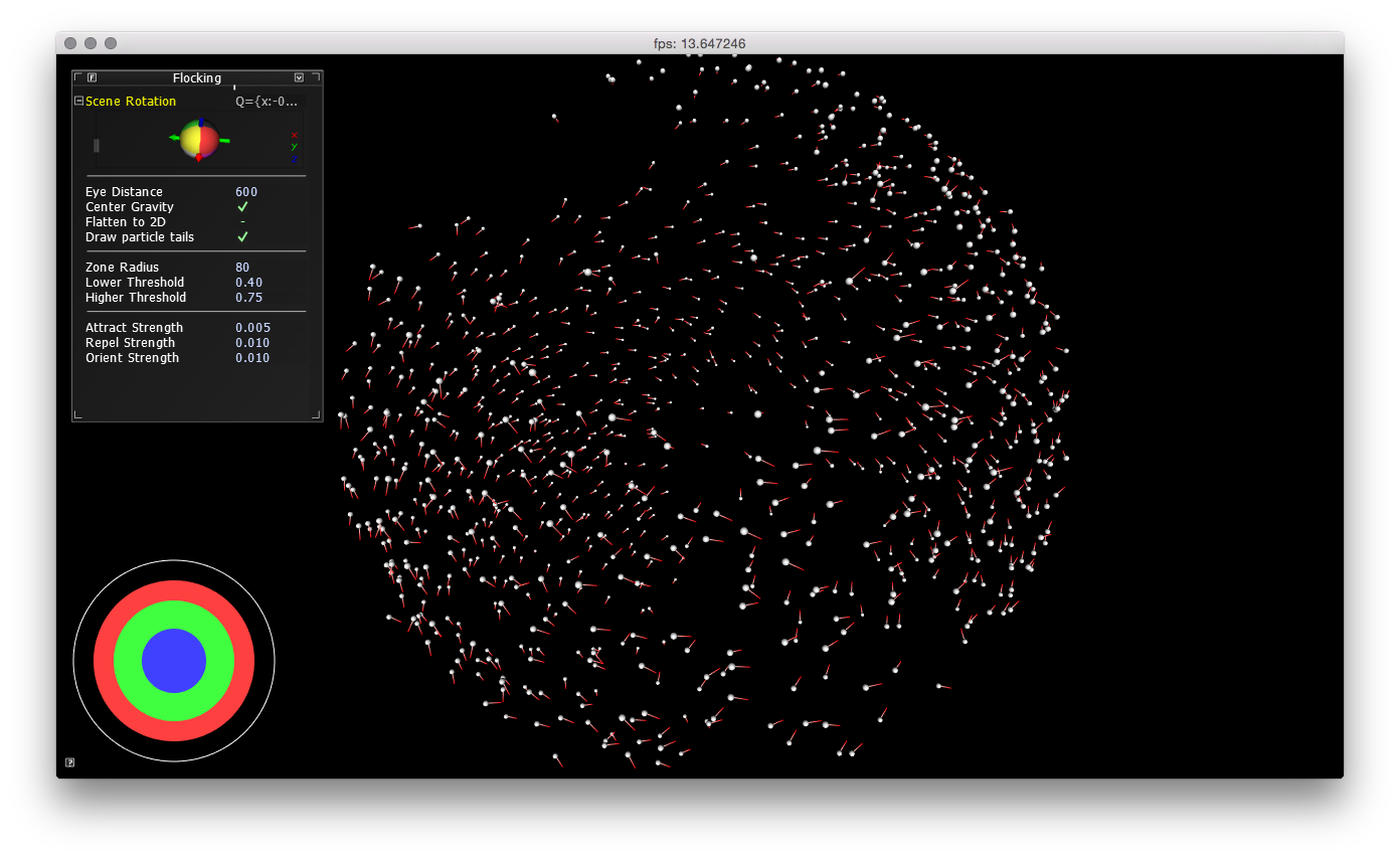Final rendition of the Cinder flocking application

Although the tutorial taught me a lot about Cinder in general and C++ and OpenGL specifically, I came to find out that the Cinder’s extension for Kinect does currently not work in the latest version. One of the reasons is, that Cinder switched from their own math library to GLM. While errors resulting from this change would be easily fixed, I also ran into other issues I was unable to resolve. Given that I knew from the start that my project would rely on the Kinect camera, I continued to work with openFrameworks.

Examples

Perlin Noise

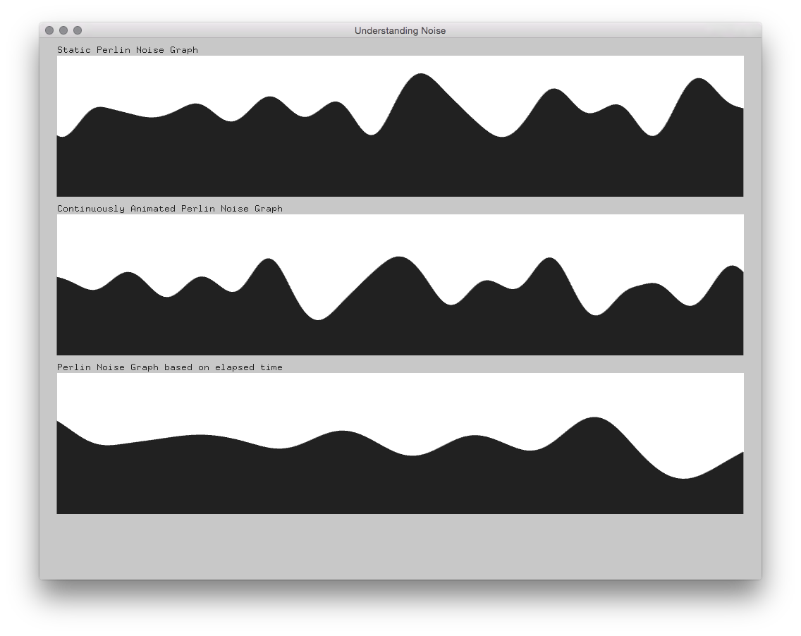
Although I worked with Perlin Noise before, I build a little graphing example to refamiliarize myself with its parameters. The result is the Understanding Noise example.

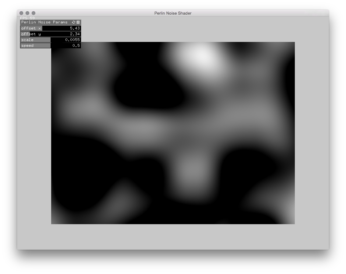
Ultimately I wanted to write a class that would output two-dimensional perlin noise pixel data. My intention was to create an alternative input for debugging, so I’d be able to work on code without having to connect a Kinect. Quickly I realized that doing the calculations and pixel buffer updates on the CPU was way to slow. So I had write a OpenGL shader program in order to generate the same output on the GPU. At first I thought, I’d find an off-the-shelf solution for this in no time. But turned out that I was either checking the wrong resources or it did not yet exist in the form that I needed it.

After doing some research and tutorials I finally managed to get it up and running. The code can be found in the Perlin Noise Shader example.

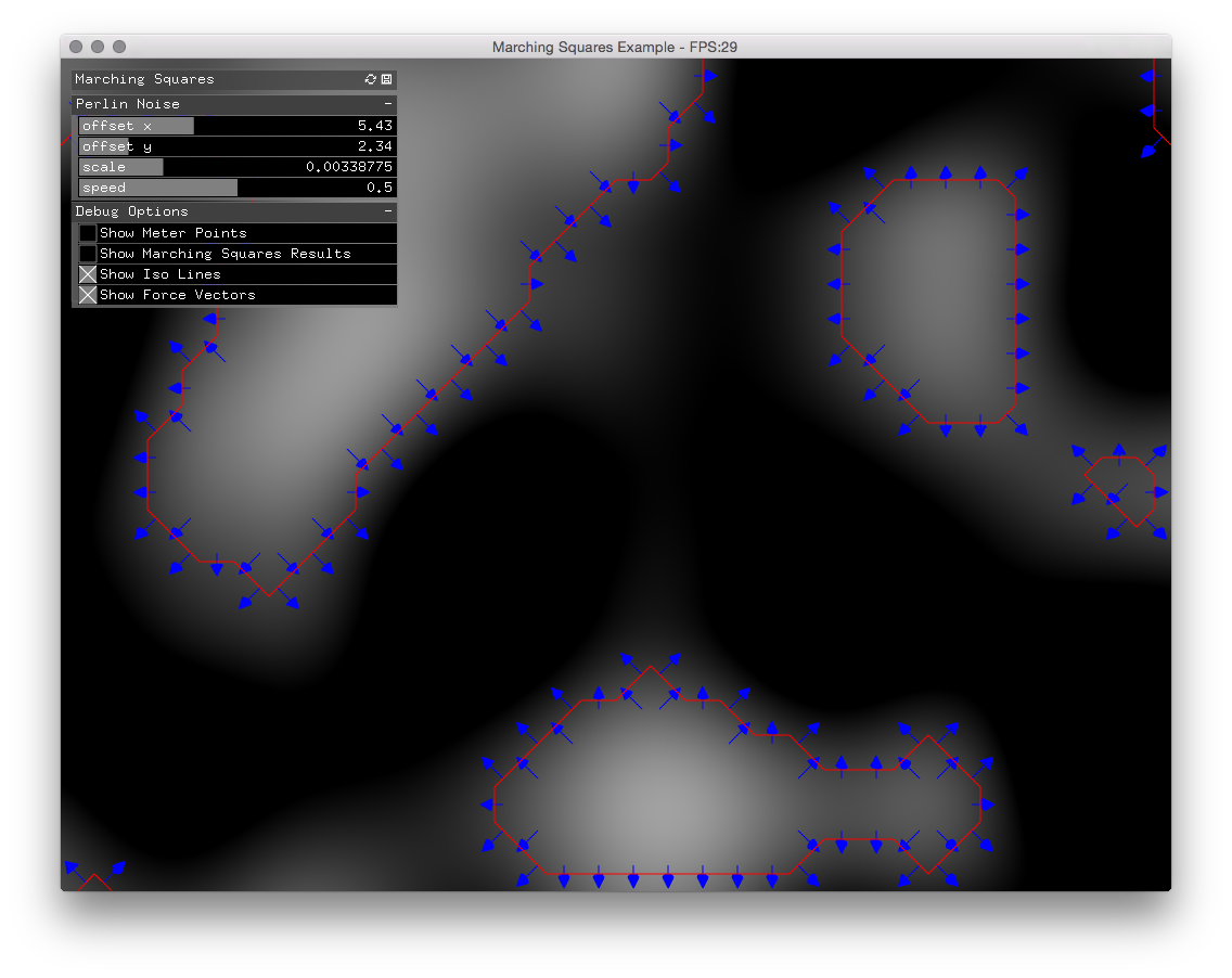
Marching Squares

In order to analyze the input from the Kinect camera and calculate the vectors pointing away from lighter (closer) areas, I resorted to the marching squares algorithm. The algorithm is used to find the contour lines in a two-dimensional scalar field. So the idea was to place a grid of measuring points on top of the Kinect pixel data and find all contour lines based on a certain threshold. From the contour lines I then calculated the perpendicular lines. These perpendicular lines I then used as vectors pointing away from white areas.

So far this solution worked out fine. But then I neeed another algorithm which would assign vector forces to all inner quadrants in my segmented input data. For this purpose I first looked into the flood fill algorithm. The problem with this algorithm was that it started from a random location inside the contour line and then iteratively looked at its surrounding segments. Since I only had forces assigned to contour segments and all of the inner segments should be derived from the closest contour vectors, this algorithm did not work out by default.

An idea was to keep track of all contour segments during the execution of the marching square algorithm. Then I’d look at all surrounding, inner segments and store them with the association to the contour vectors. Then I’d calculate the vector based on all associated contour vectors. This then would yield another list of segments which run through the same routine. This would continue until there were no inner segments left. Although possible in theory, the implementation proved to fairly complex. And since I needed this code to run fast and efficiently at at least 30 frames per second, I looked into alternatives.

My next candidate then were path finding algorithms, namely Dijkstra’s algorithm and A* search algorithm. The idea here was to find the closest contour segments for each inner segment. Though it would work to ‘walk’ from inside segments towards contour segments then the problem remained to assign forces from the outside segments to the inner ones. After some experimentation, I became convinced that my initial instinct to choose the marching square algorithm was flawed and the reason for the problems I was running into. So I went back to my initial problem and searched for different solutions.

Vector Field

After my problems with the marching squares approach, another solution turned out to be right in front of me all along: vector fields or flow fields. Although I did not immediately find the reference with which I was working from the start. Before that I found an example for openFrameworks of a course on algorithmic animation by Zach Lieberman. In the end I arrived back at Daniel Shiffman’s book The Natur of Code where in the chapter 6 on Autonomous Agents he writes at length about Flow Fields.

After implementing my own vector field from scratch, based on the two aforementioned resources, I was finally on the right track. The solution proved to be flexible and with very good performance. The version demonstrated below is already a little bit more complex than the Simple Vector Field example provided in my repository. The main difference is that the video also demonstrates a working particle system that is connected to the output of the vector field.

After discovering Shiffman’s book I started a separate repository for my ‘The Nature of Code’ implementation for openFrameworks. This repository is very incomplete, since it only features some code example from chapter 6. But I’ll definitely return to this repository to continue implementing other examples. In case you’re looking for more complete implementations there are many more people who approached this endeavour more thoroughly.

Homography

After having figured out how to generate perlin noise and use it as my input for the vector field, I had to face the issue of how to extract the Kinect depth data only in the area I was projecting onto. I needed a solution that I could easily adjust to different setups and locations. Otherwise I would have to change my code everytime I use a different projector or setup the installation in a different space. The solution I ended up using was a homography, also called projective transformation.

The advantage of using this transformation is, that any polygon described by four points can be transformed into another polygon of four points. This property really worked in my favor, because I could not only extract a specific area in my depth data but also straighten the source data into a rectangle. This rectangle then had the same properties as the pixel image generated by my perlin noise shader programm. Thereby the two methods were became interchangeable which allowed me to easily switch between the two at runtime.

The image below is a screenshot of my OpenCV Homography example. This example shows the a slightly more complex application of the principle than I originally needed. There are two homography transformations applied where the output of the first transformation becomes the input of the second transformation. I wrote this slightly more complex example – including the custom UI elements to define the homography points – because I felt that this would visualize the power of this mathematical principle most clearly.

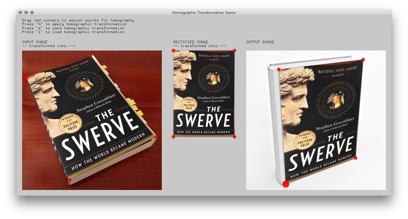
The example is based in the openFrameworks addon ofxCv by Kyle McDonald, who wrote a fast and accessible implementation of the homography transformation.

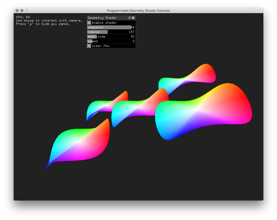
Programmable Geometry Shader

In preparation for the final visualization of the particle system, I started to delve deeper into OpenGL shader programming. Of specific interest to me was the geometry shader stage in the graphics pipeline. It would allow me to handle only simple point data on the CPU and generate complex parametrized geometry on the GPU. Therefore I came up with this Geometry Shader example. On the repository page I also list the resources I used when creating this example.

Working Prototype

This video show a complete walkthrough of the setup configuration and the interaction between the fabric and the projection. The first part demonstrates the configuration. The infrared (IR) needs to masked during the setup of the homography transformation in order to get a better camera image without the pseudo-random IR pattern in it. Once the setup is finished I show the mapping of the 3D depth data to the projection by projecting the depth buffer onto the fabric. This demonstrates how the interaction with the fabric is mapped to the depth data visually. In the last part I demonstrate how the depth data is powering a particle system through the use of a vector field. The particle system of the projection is not the final visualization.